

RIA Result Calculator – Radioimmunoassay Standard Curve & Sample Concentration
RIA Calculator – Introduction
Understanding the principles, methods, and practical use of Radioimmunoassay data analysis.
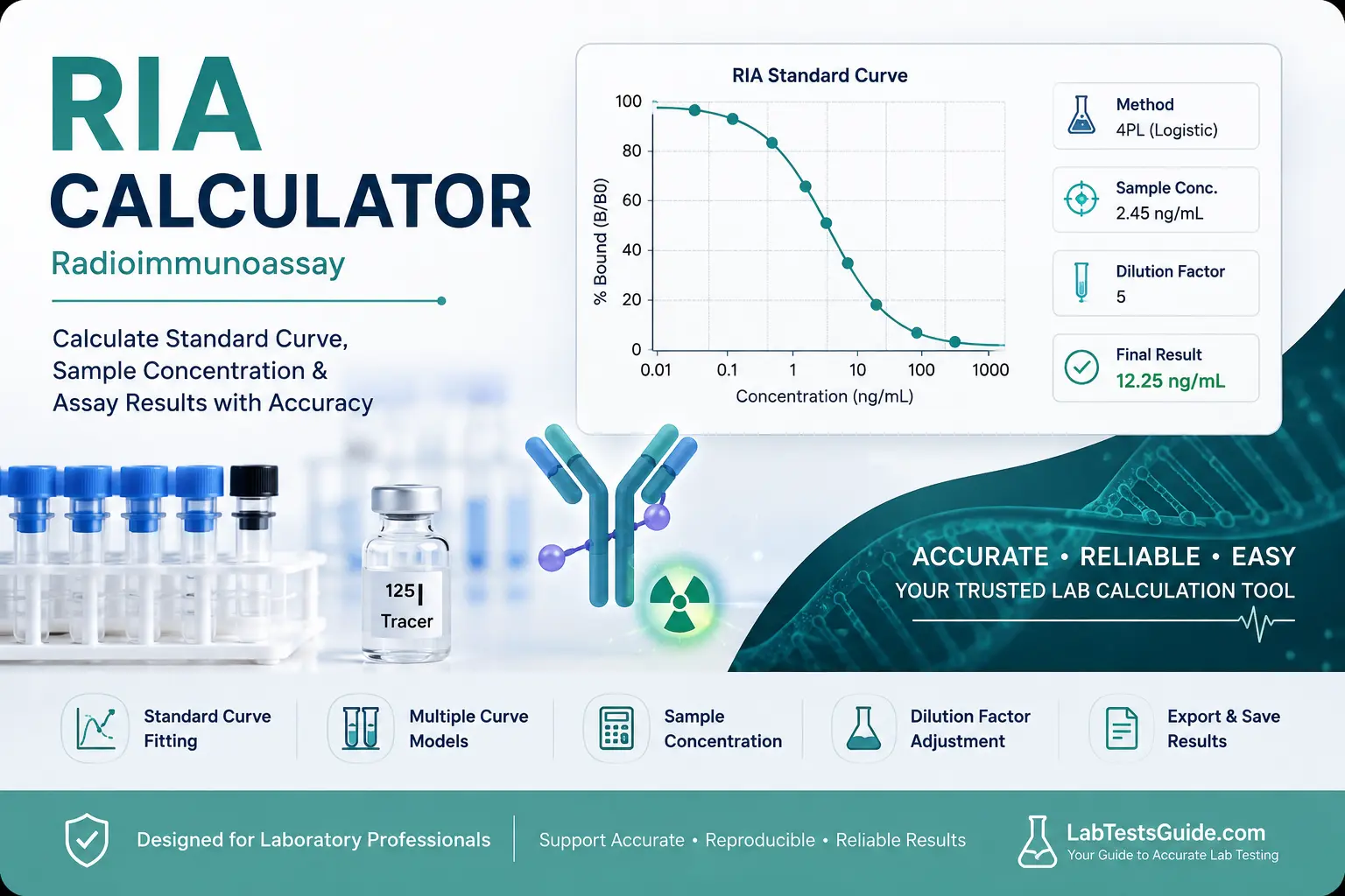
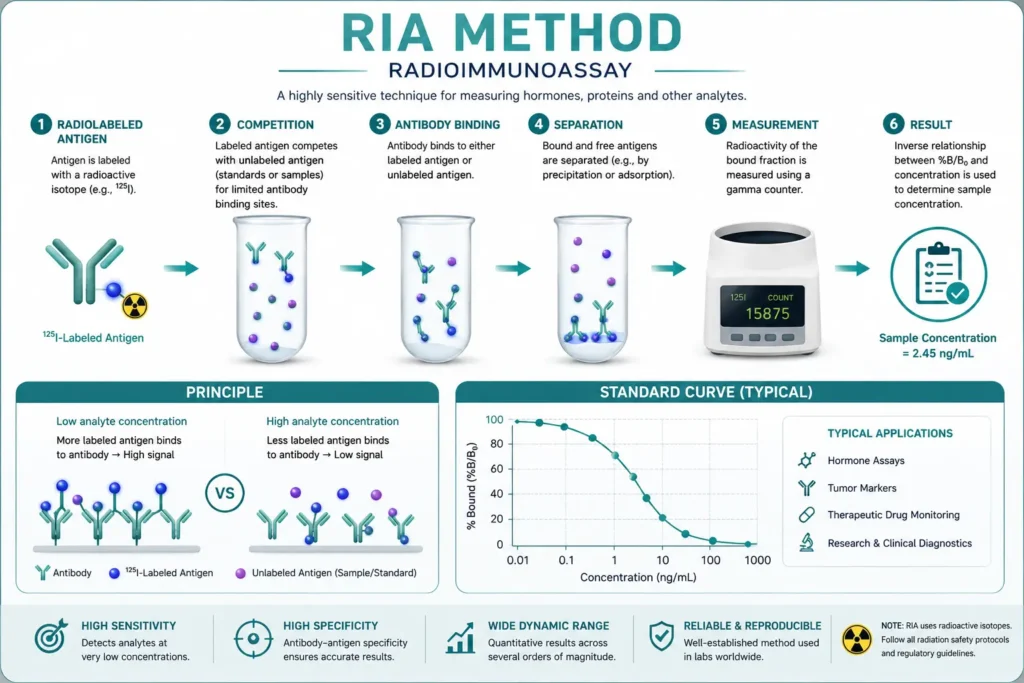
Radioimmunoassay (RIA) is a highly sensitive in vitro assay technique that uses radioisotope-labeled antigens (or antibodies) to measure the concentration of specific analytes (hormones, drugs, proteins) in biological samples. It relies on competitive binding between a known quantity of labeled antigen and the unknown antigen in the sample for a limited number of antibody binding sites.
Developed by Yalow and Berson in the 1950s, RIA remains a gold standard for endocrinology, pharmacokinetics, and clinical diagnostics due to its exceptional sensitivity and specificity.
An RIA calculator automates the entire data reduction workflow:
- Normalization: subtracts NSB (non‑specific binding) and calculates B/B₀ or %B/T.
- Curve fitting: fits a 4‑parameter logistic (4PL) or 5PL model to the calibrator data.
- Interpolation: converts unknown sample signals into concentrations via the standard curve.
- QC & validation: flags outliers, calculates recovery, CV%, LLOQ/ULOQ, and extrapolation warnings.
- Reporting: generates tables, graphs, and exportable results for clinical documentation.
RIA data analysis is essential in:
- Endocrinology: thyroid hormones (T3, T4), insulin, cortisol, growth hormone.
- Pharmacokinetics: drug concentration monitoring (digoxin, theophylline).
- Clinical diagnostics: tumor markers (AFP, CEA), vitamin D, ferritin.
- Research: cytokine measurement, peptide/protein quantitation in biological fluids.
- Assay validation: establishing LOD, LOQ, linearity, and spike recovery.
Known concentrations (including zero calibrator B₀) are measured in replicates.
Bound radioactivity (B) is separated from free (F) using precipitation or separation techniques.
A non‑linear regression (4PL/5PL) is fitted to the dose‑response data (conc. vs. normalized signal).
Each unknown’s signal is back‑projected onto the curve to obtain its concentration.
Multiply by the sample dilution factor to report the original concentration.
Results are validated with QC checks (recovery, CV, range) and reported with units.
Several mathematical approaches are used to model the RIA standard curve:
Simplest model, assumes a straight‑line relationship between concentration and response. Rarely adequate for RIA.
Log10(concentration) vs. response – linearizes the mid‑portion of the curve.
Logit transformation of binding data (ln[Y/(100‑Y)]) against log concentration. Classic RIA method.
Y = D + (A − D) / [1 + (X/C)B]. The industry standard, handles sigmoidal shape with upper/lower asymptotes.
Adds an asymmetry parameter (E) to the 4PL model, improving fit for asymmetric curves.
- Assay protocol details: RIA type (competitive/non‑competitive), isotope, and unit system.
- Total counts (T): measure total radioactivity added to each tube.
- NSB replicates: non‑specific binding tubes (antibody‑free).
- B₀ replicates: zero‑standard (maximum binding) tubes.
- Standards data: at least 6‑8 calibrator concentrations with replicates (duplicates or triplicates).
- Unknown sample replicates: each sample should have 2‑3 measurements for CV QC.
- Dilution factors: for each sample that was pre‑diluted before assay.
| Input | Description | Clinical Significance |
|---|---|---|
| T (Total) | Total radioactivity added (counts per minute). | Normalization factor for B/T% calculations. |
| NSB | Non‑specific binding – counts from tubes without antibody. | Subtracted to correct for background matrix effects. |
| B₀ | Max binding (zero calibrator) – highest expected signal. | Used as denominator for B/B₀ and %B/B₀. |
| Standards | Known concentrations with measured responses. | Construct the calibration curve; define LLOQ/ULOQ. |
| Unknowns | Sample signals (CPM/CPS) with replicates. | Interpolated to obtain clinical concentration. |
| Dilution factor | Pre‑assay dilution applied to the sample. | Final concentration = interpolated × dilution. |
Counting units: CPM (counts per minute) is standard; CPS (counts per second) can be converted by ×60. Raw counts require known counting time.
Concentration units: Common formats include pg/mL, ng/mL, µg/mL, IU/mL, pmol/L, nmol/L. The calculator does not auto‑convert between mass and molar units unless molecular weight is provided.
Normalization: %B/B₀ = (B − NSB) / (B₀ − NSB) × 100 is the most widely used response metric. %B/T is an alternative for certain protocols.
Dilution correction: Always apply the sample dilution factor after interpolation. Serial dilutions can be calculated cumulatively.
Radioimmunoassay (RIA) Data Analysis Platform
Clinical Grade Data Reduction • 4PL Fitting • Responsive Engine
| ID | Conc | Rep 1 | Rep 2 | Rep 3 | Mean | CV% | Y | Rec% | |
|---|---|---|---|---|---|---|---|---|---|
| — | — | — | — | ||||||
| — | — | — | — | ||||||
| — | — | — | — | ||||||
| — | — | — | — | ||||||
| — | — | — | — | ||||||
| — | — | — | — |
| Sample ID | Rep 1 | Rep 2 | Rep 3 | Mean | CV% | Y | Interp | Dilution | Final Conc | Status | |
|---|---|---|---|---|---|---|---|---|---|---|---|
| — | — | — | — | — | — | ||||||
| — | — | — | — | — | — | ||||||
| — | — | — | — | — | — |
Radioimmunoassay (RIA) Calculation Guide
Clinical and laboratory documentation for four-parameter logistic (4PL) regression, quality metrics, and sample interpolation.
How to Use the RIA Calculator & Data Entry
- Select the detection unit: CPM (Counts Per Minute) or CPS (Counts Per Second).
- Enter total counts (T), non-specific binding (NSB), and zero standard (B₀) replicates.
- Input known standard concentrations alongside replicate response values (Rep 1, Rep 2).
- Add unknown sample identifiers and replicate raw count values.
- Set the appropriate Dilution Factor (DF) for each sample (default is 1 for undiluted).
- System auto-calculates mean counts, %CV, binding metrics, and final corrected concentrations.
Understanding the Standard Curve & Results
RIA assays utilize competitive binding mechanisms. The calculator transforms raw response metrics and applies non-linear regression analysis.
- %B/B₀ Transformation: Normalized competitive response calculated as:%B/B₀ = [(Mean CPM – NSB) / (B₀ – NSB)] × 100
- Net Counts (B – NSB): Absolute specific binding without normalization.
Interpolation is executed using the 4-Parameter Logistic (4PL) model:
- A: Minimum response (high dose asymptote)
- B: Hill slope factor
- C: IC₅₀ / EC₅₀ concentration
- D: Maximum response (zero dose asymptote)
Dilution Factors & Example Calculation
When samples exceed the Upper Limit of Quantification (ULOQ), dilution is required. The final concentration is calculated as:
Example: A 1:5 dilution has a DF = 5. If interpolated value = 12.4 ng/mL, final value = 62.0 ng/mL.
| Step | Parameter | Value |
|---|---|---|
| 1 | NSB Mean | 350 CPM |
| 2 | B₀ Mean | 12,500 CPM |
| 3 | Net B₀ (B₀ – NSB) | 12,150 CPM |
| 4 | Sample Mean (Raw) | 6,425 CPM |
| 5 | Calculated %B/B₀ | 50.0% |
| 6 | 4PL Back-Calculated Conc. | 4.82 ng/mL |
RIA Quality-Control (QC) Considerations
| QC Parameter | Clinical Definition | Acceptance Criteria |
|---|---|---|
| Blank / NSB | Non-specific binding of tracer to tubes/wells without antibody. | < 5% of Total Counts (T) |
| Zero Standard (B₀) | Maximum binding capacity in the total absence of unlabeled antigen. | 30% – 60% of Total Counts (T) |
| Controls (QC Low/High) | Serum matrix samples with established target values. | Within ±2 SD of target value |
| Replicates & %CV | Precision evaluation across duplicate or triplicate pipetting. | %CV ≤ 10% (Standards & Samples) |
| Outliers | Replicates with high variance due to pipetting/decanting errors. | Exclude if %CV > 15% and rerun |
| Curve Fit Metrics | Goodness-of-fit parameters evaluated for non-linear regression. | R² ≥ 0.985; Back-fit recovery 80–120% |
Troubleshooting, Limitations & Method Comparison
- Unit Mismatch: Combining CPM data with CPS without factor conversion (1 CPS = 60 CPM).
- Uncorrected NSB: Subtracting NSB from sample counts without subtracting it from B₀.
- Extrapolation Beyond Range: Reporting concentrations below LLOQ or above ULOQ.
- Hook Effect: Extremely high analyte concentrations yielding falsely lower response signals.
- Calculations assume uniform radioisotope decay across all tubes within a single batch run.
- The 4PL algorithm requires a minimum of 4 distinct standard concentration points to fit parameters accurately.
- Inadequate for non-competitive (sandwich-type) radiometric assays without model adjustment.
| Feature | RIA Analysis | ELISA Analysis |
|---|---|---|
| Signal Inverse | Higher Conc = Lower CPM | Higher Conc = Higher OD |
| Primary Model | 4PL Competitive | 4PL / 5PL Direct |
| Decay Correction | Required (Isotope half-life) | Not applicable |
Frequently Asked Questions
References and Sources
- Berson SA, Yalow RS. – Radioimmunoassay of peptide hormones. Journal of Clinical Investigation. | Important foundational work on peptide-hormone RIA methodology. – (accessed on Aug 22, 2026)
- Chard T. An Introduction to Radioimmunoassay and Related Techniques. 3rd ed. Elsevier; 1995. | An Introduction to Radioimmunoassay and Related Techniques – (accessed on Aug 22, 2026)
- Bikash Dwivedi. Radioimmunoassay (RIA): Principle, Procedure, Results, Uses | Microbenotes.com – (accessed on Aug 22, 2026)
- B. Linkitha. Radio immunoassay (RIA) Advanced Pharmaceutical Analysis – PPTX | Slideshare.net – (accessed on Aug 22, 2026)
- Farbwerke Hoechst A.G., Frankfurt am Main (Germany, F.R.). Radiochemisches Lab. Radioimmunoassay (RIA), a highly specific, extremely sensitive quantitative method of analysis | International Atomic Energy Agency (IAEA) – (accessed on Aug 22, 2026)
- Ayush Chauhan. Radioimmunoassay (RIA) Guide: Principles & Applications flabslis.com – (accessed on Aug 22, 2026)
- Prince Kumar – Understanding Radio Immuno-Assays: A Guide to RIA Techniques | Environmental Studies (EVS) Institute – (accessed on Aug 22, 2026)
- PubMed – Radioimmunoassay procedure for quantitating bacterial antibody in human sera | DOI: 10.1016/0022-1759(77)90142-9 – (accessed on Aug 22, 2026)
